Time series

People live and all events happen in time dimension. Time series data point is a combination of a timestamp (t), the actual value (v), and quality (q). Time series data point X can be presented as equation:

       X = (t, v, q) 

Sensor value is a typical time series that may be of different type; discretely changing or expected to change continuously. The data values can be collected with regular time intervals or irregular that means the value is recorded whenever it is changing. Value contains also quality information that describes how reliable the value is. Value data type may be numerical, enumerated, string, timestamp, array of previous, or blob.

Another type of time series data is event. Event represents typically a time period with start and end time, and then it may contain various other attributes. Examples of events are such as run period of a motor, signal exceeding an alarm limit, manufacturing a discrete product, and grade run or other process phase in a production line.

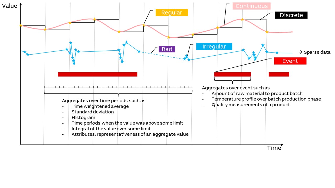
Time series data can be consumed by the applications e.g. in the following ways:

• Real-time data stream, e.g. to process and event monitoring
• Historical raw data, e.g. to trend plots
• Aggregated over time periods, e.g. hourly energy consumption
• Aggregated over events, e.g. how much of particular raw material or energy has been consumed to produce a piece of a product.

Aggregated data may also be more complex such as histogram or time slices when the value has been over some limit, or it may be freely calculated from one or more time series data, and it may contain attributes such as representativeness describing the reliability of the value.

To make it possible to handle the time series data streams, there must be some metadata to describe the semantics. Metadata is used to describe the identification of the data stream, where it belongs in bigger picture, and engineering attributes such as description of the time series, value data type, value unit, min/max limits for the value, how it is collected from the source, which kind of preprocessing is performed before storing, where it is stored, and which kind of automated aggregation is wanted to perform.

For describing the meta data there are several information model concepts in ABB Ability™ History: Tag, Variable and Equipment Model.

Aggregates and filters

Raw sensor value is the bases for collecting time series data, but very frequently applications prefer using aggregated data. Aggregation means filtering the raw time series data with some function such as averaging. Typical filter is constructed from the function and time period such as AVG10min, which means that the raw time series data is divided in 10 min slots and AVG (= time weighted average) is applied to the 10 min data sets and the results is time stamped with the start time of the 10 min time period.

Raw data as well as aggregated data contains always the value, timestamp and quality status. It is important to understand how the timestamp and quality status are formed in the aggregation in addition to the actual value. Also so called interpolation rules are affecting to aggregated values, especially if the quality of the source values are changing.

The following table gives basic rules for the interpolation.

• Left value: source value before the interpolation time
• Right value: source value after the interpolation time

The following pictures briefly present the ABB Ability™ History transformation types. Each type uses the same CurrentHistory data as the transformation base. The graphs show the source data and the results. The markers in the curves describe the actual data points. The vertical lines in the pictures separate periods.

Averages

There are 3 filters to show averages in ABB Ability™ History: Arithmetic Average (AAVG), Time Weighted Average (AVG), and Raw Time Weighted Average (AVGRAW).

Arithmetic Average is a sum of values divided by the number of values. The time-weighted average is the average of the valid source values that are weighted by the time before the next value. As weights are used, the values are in effect within the period. In other words, the time-weighted average considers the time interval between data points. Raw Time Weighted Average presents the average of all regardless of the quality status of the source values.
Averaging is either linear or discrete according to the source data. The result is stored as a floating-point number.

The graph presents all 2 filters on the same dataset:

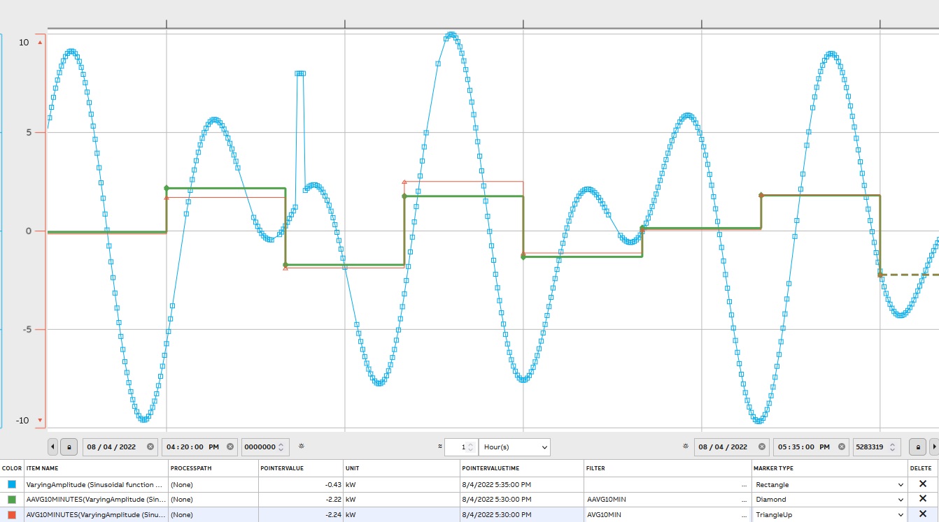
On the graph, the difference between Arithmetic Average (AAVG) and Time Weighted Average (AVG) can be noticeable for the same dataset.

Deviation

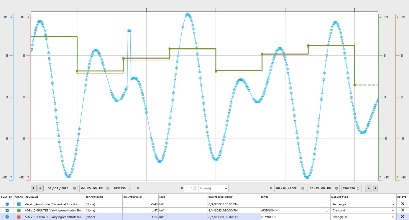
There are 3 filters for finding deviation in ABB Ability™ History: Arithmetic Deviation(ADEV), Arithmetic Deviation of Entire Population(ADEVP), and Time Weighted Deviation(DEV). The standard deviation is a measure of how spread out numbers are. The standard deviation formula for continuous function deviation is applied.
Formula:

                σ= √((∑(xi- μ)^2 )/N)

σ - population standard deviation
N - the size of the population
xi - each value from the population
μ - the population mean

The result is stored as a floating-point number. The graph presents 2 filters on the same dataset:

Variance

The measure of dataset variability is the variance. It tells the degree of spread of data.
The population variance is expressed as:

               σ^2=  (∑(xi- μ)^2 )/N

σ^2 - population variance
N - number of values in the population
xi - each value from the population
μ - the population mean

As it can be noticed that deviation and variance reflect variability in a distribution. However, the main difference between the variance and standard deviation is the units. Standard deviation is in original value units (e.g. m), while variance is expressed in the square of the units of values(e.g. m^2).
There are the arithmetical variance (AVARIANCE) and the arithmetic variance of the entire population (AVARIANCEP)

Median

Two Median filters are available: AMEDIAN is the arithmetic median (the middle number). MEDIAN is the time weighted median value. MEDIAN takes an optional parameter 0..1 that indicates the percentile (its default value is 0.5). For example MEDIAN(0.75) takes the third quartile.

Arithmetic Mode

To determent arithmetic mode (the most frequent value) use AMODE

Calculation

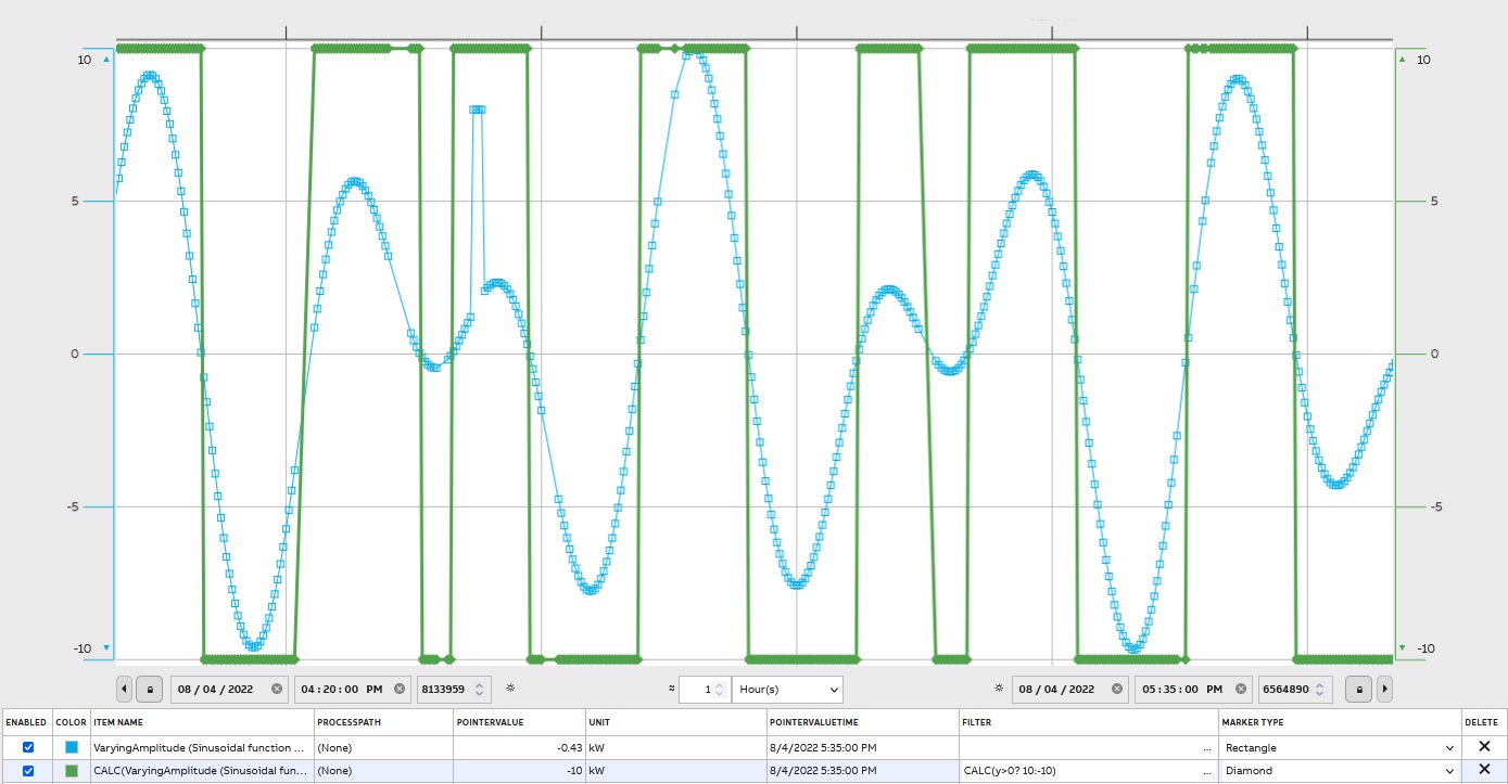
Users can define calculation by using CALC, e.g. CALC(y*2) which returns doubled values, CALC(y > 0 ? 10:20) returns 10 if y > 0, otherwise 20.On Filter page( https://docs.cpmplus.net/docs/using-filters) Supported constants and functions can be found.
The graph presents result for CALC(y>0 ? 10:-10):

Unit Conversion

Values can be converted between different units by CONVERT, e.g. CONVERT(hp) which presents values in horse powers instead kilowatts:

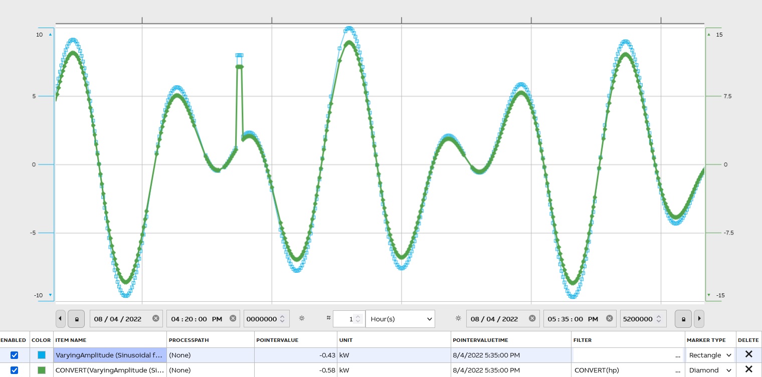
History contains a unit conversion table with 500 most common units, and it can be extended.

Cumulative Sum

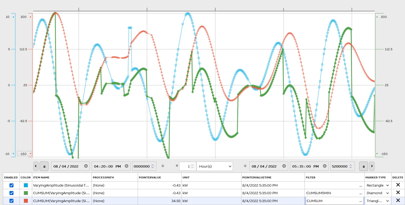
Cumulative sum (CUMSUM; CUMSUMTODOUBLE, convert values to double) is used to display the total sum of data as it grows with time. The graph compares CUMSUM and CUMSUM5MIN:

Delta and Range

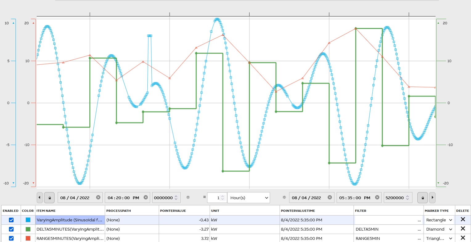
Delta (DELTA) is a difference between the last value in the period and the first: D =xlast-x1
The range (RANGE) is a difference between the maximum value in the period and the minimum: R = Xmax-Xmin.

To compare the two

Duration Filter

To find duration use DUR, DURG for a good duration, and DURI for an invalid duration. Duration is the time period the value is in effect, i.e. before there is the next value. It can be used e.g. to count how long the motor was running.

Time Integral

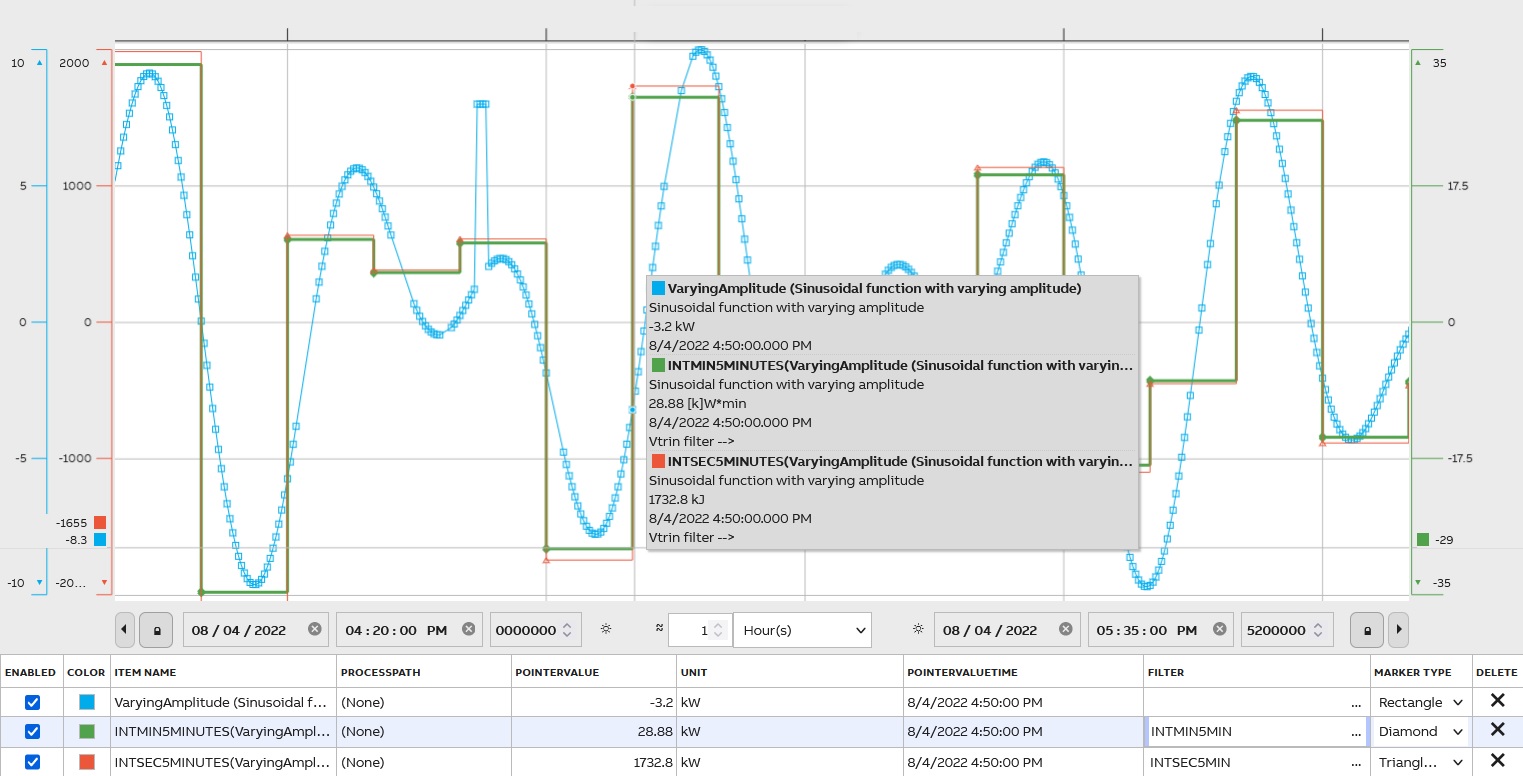
There are 3 options to reflect the time integral in seconds (INTSEC), in minutes (INTMIN), and hours (INTHOUR). At the lowest transformation level, the result is the time integral of the valid source values over the period, using seconds or hours as the time unit (separate transformation types and result tables). At higher levels, the transformation type sum is applied. The result is stored as a floating-point number.

MAX and MIN

MAX The largest valid value from the set of source values, which includes the values within the period and the interpolated values at the beginning and the end of the period. If more than one equal maximum values exist, the first (oldest) one of them is used.

MIN The smallest valid value from the set of source values, which includes the values within the period and the interpolated values at the beginning and the end of the period. If more than one equal minimum values exist, the first one (oldest) of them is used.

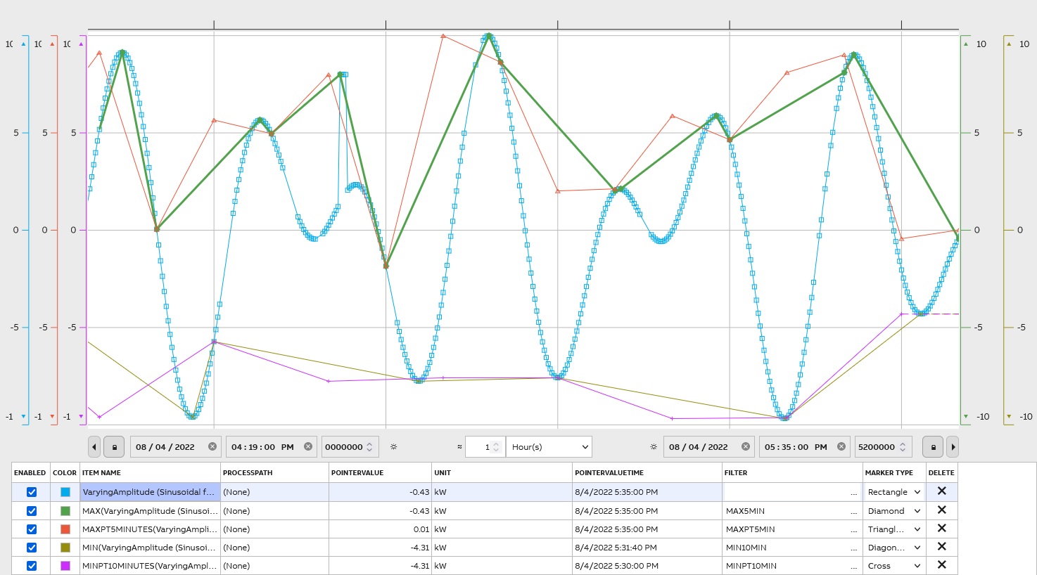
To make TimeStamp is PeriodTime use MAXPT and MINPT. It means that these filters indicate points on :00, :10, :20, :30, etc, regardless of the start time.

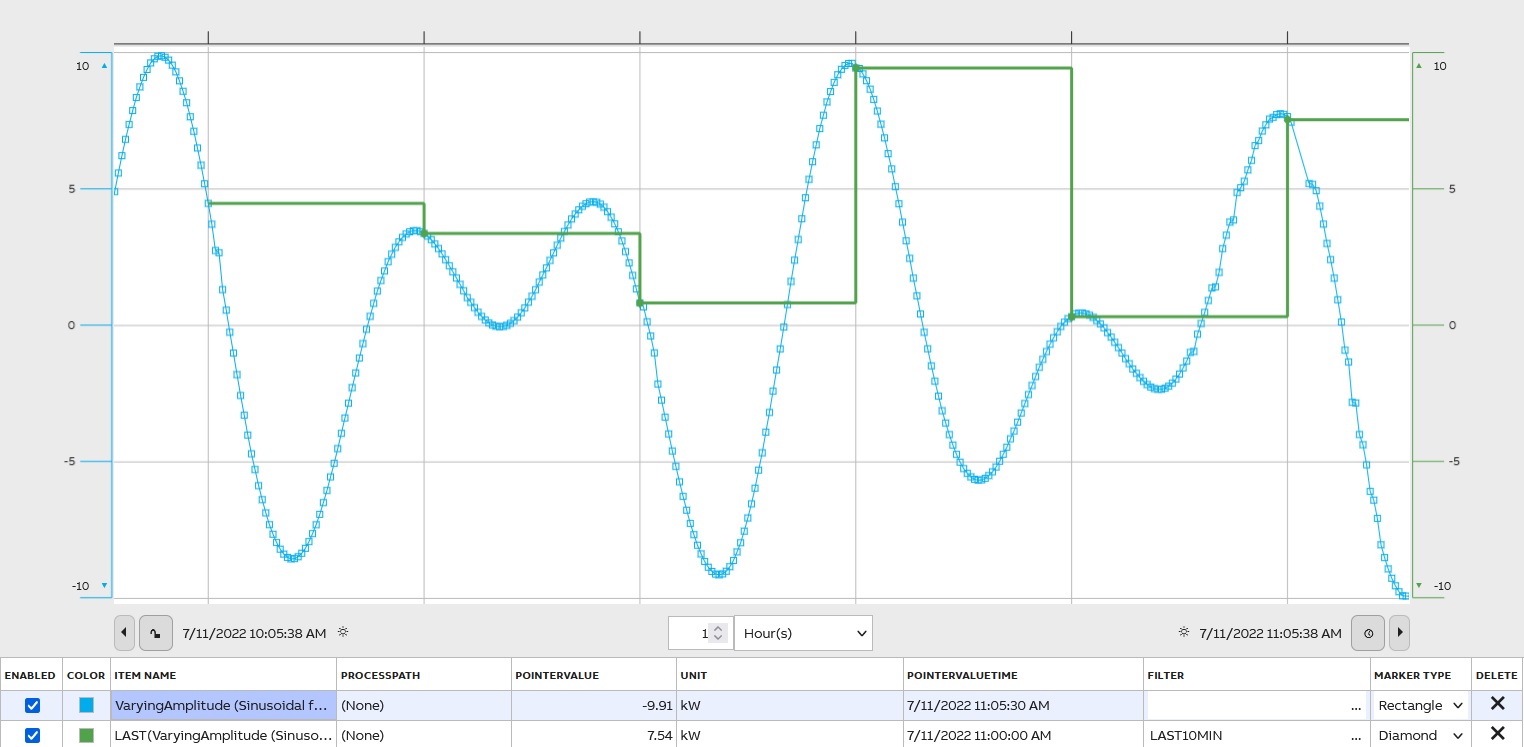
First and Last Value of a Period

To indicate the first and the last values of a period the FIRST and the LAST filter are used. Usually, the value is interpolated.

Sum of Values

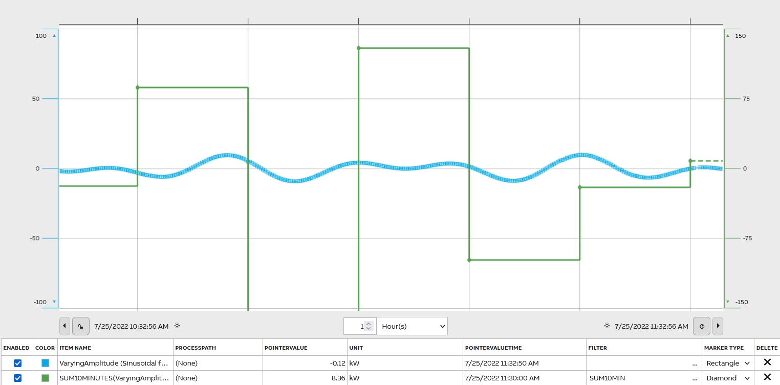
There are several filters to present the sum of values: SUM(Sum of Values Within a Period), SUMRAW(Ignoring the Invalidity of Values, even invalidity caused by HSLIS, however, see also the release notes of bugfix WI#55837 from year 2022), SUMTODOUBLE(sum is presented in double if it has the risk of overflow). Sum The sum is counted from all values having non-zero representativeness within the period. The raw sum is a sum of all source values regardless of validity and representativeness within the period. The result is stored as a floating-point number.

Operating Time

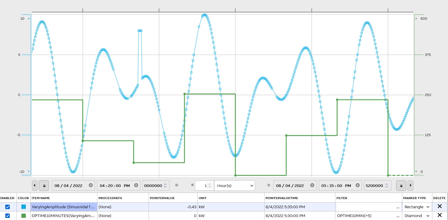
At the lowest transformation level, the value is the time of the period, for which the source variable is valid and stays in its defined range (analog) or state (binary). The value is the time the source value curve is above the trigger limit. At higher levels, this transformation operates like a sum. Requires a parameter, e.g. OPTIME10MIN(>5) calculates the time the value has been greater than 5. The filter name is OPTIME. The result is stored as a floating-point number. The unit of the value is an hour:

Percentage of samples

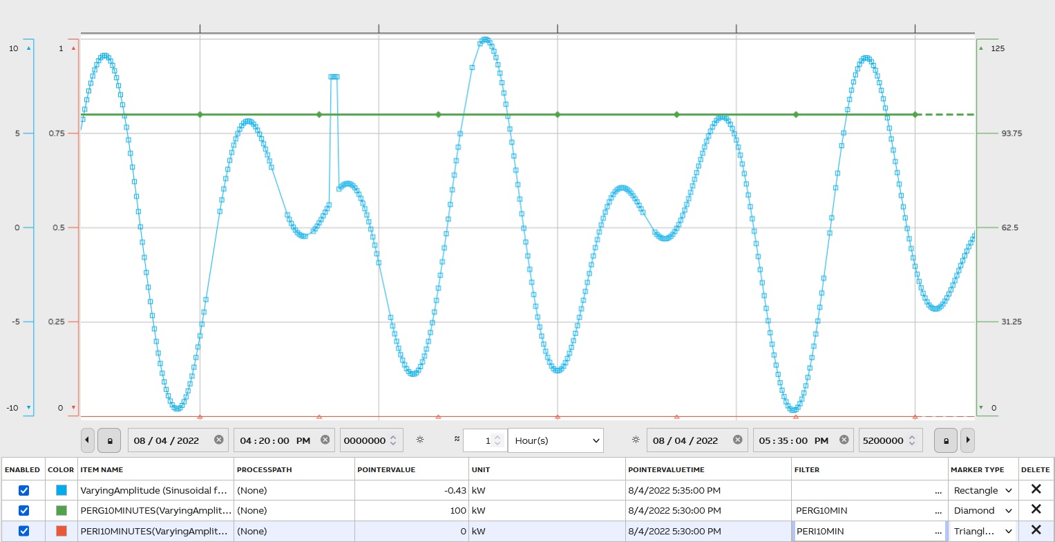
To reflect the percentage of good or invalid samples within the time period in the format from 0 to 100% use PERG and PERI respectfully.

Skip

Skip and select period values SKIP(initial_skip, value_skip, [value_include])
initial_skip – period to start, e.g. 3 skips 3 periods
value_skip – how many periods to skip between the selected ones, e.g. 2 skips 2 periods and selects every third
value_include – optional, how many values to return before the next skipped batch

SKIP can only be used after some other periodical filter, not with raw value query, e.g. AVG1HOUR|SKIP(0, 3) selects every 4th-hour average value.
An example compares AVG5MIN and AVG5MIN|SKIP(3,2):

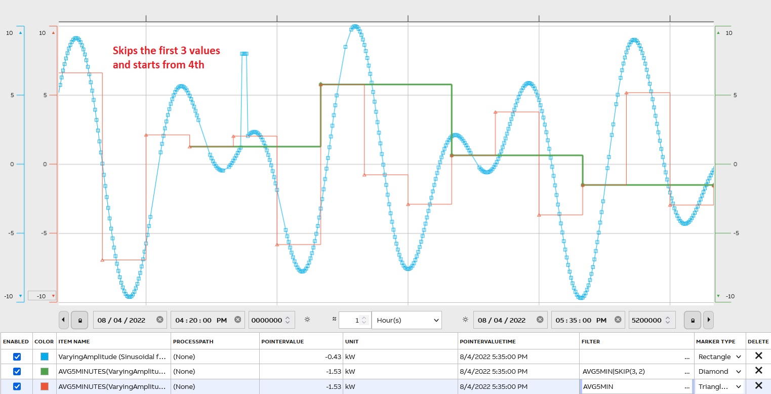
The first 3 values are skipped and after every 3rdvalue is shown (2 skipped).

Startup Count

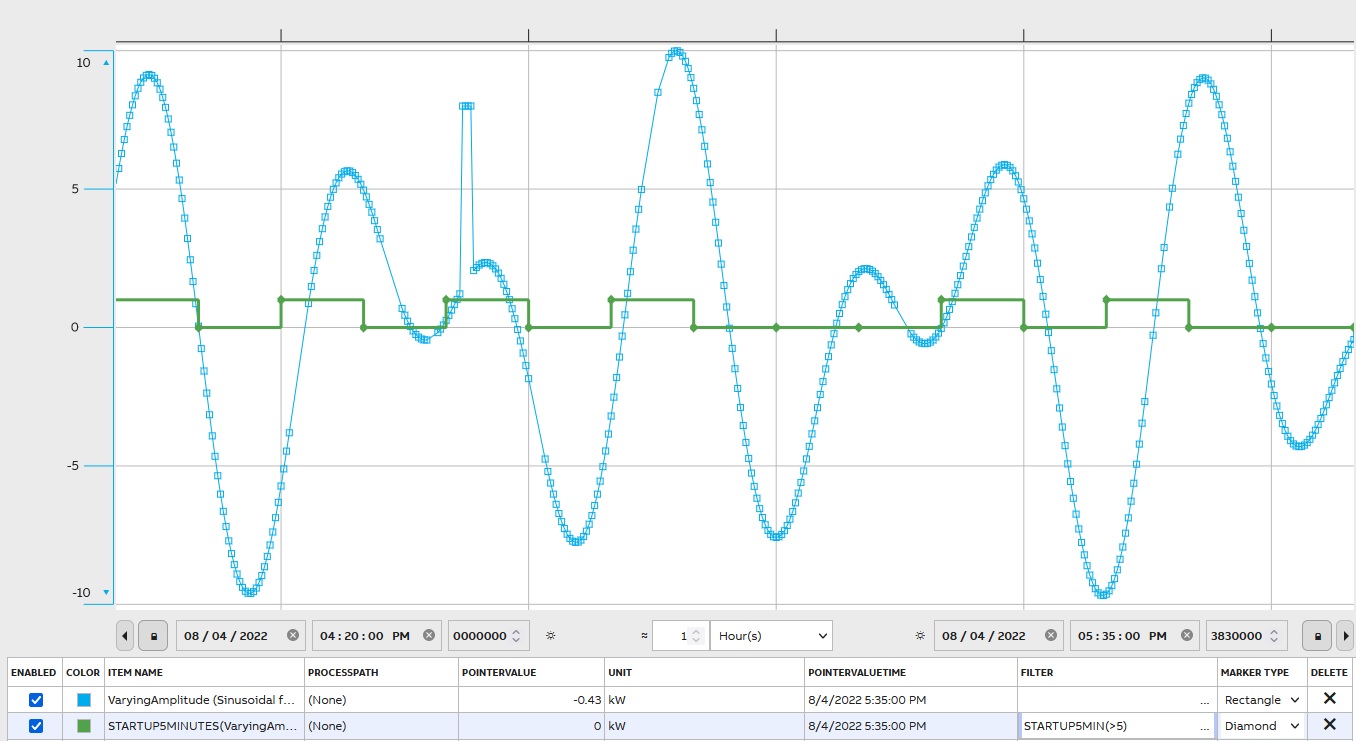
Startup Count - requires a parameter. E.g. STARTUP5MIN(>5) calculates the number of occurrences the value has increased from less than or equal to five to greater than five:

Count Samples

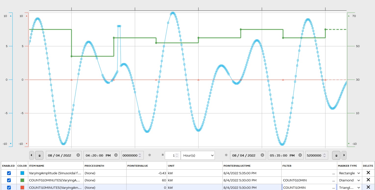
To determent, the number of values in the period use a filter COUNT. To count only good samples – COUNTG; invalid samples – COUNTI; to count questionable samples – COUNTQ; and for substituted values – COUNTS. All data counted within the period.

When

To fetch values with conditions use WHEN.
There is a detailed description on the Filters page(https://docs.cpmplus.net/docs/using-filters)

Histogram Graph

The histogram graph of input data is a bar representation of this data. Often data is classified into range groups and count how many data points belong to each group. For example, histograms are useful for analyzing change over time, and reflect a number of elements that fall into the percentage range (e.g., 0-10%, 10-20%, 20-30%, etc.). Filter name is HISTOGRAM.

A Fast Fourier Transformation

It is an implementation of an algorithm that computes the discrete Fourier transform of a sequence and presents the results on the frequency axis. The filter’s name is FFT.

Online Archiving

ABB Ability™ History supports online archiving for the time series history data for all history table types, i.e. raw histories, aggregate histories, events, or some application specific histories. The length of the archiving can be freely defined and is limited only by the available storage space. Online archiving is superior compared to some traditional archiving methods.

Lets take a look at the use cases, why archiving is typically needed:

1. Data Preservation: Archiving ensures that critical data is preserved over the long term, protecting it from accidental loss or corruption. This is handled by redundancy and daily backups in the online archiving.
2. Compliance: Many industries are subject to regulations that require them to retain records for a certain period. Archiving helps meet these legal requirements. Online archiving provides easy access to all historical data directly from the UI without any additional tasks.
3. Efficiency: Traditionally by moving older, less frequently accessed data to archives, companies can improve the performance of their active systems and reduce storage costs. Online archiving provides best performance to recent data as well as to old data, no matter what is the storing period.
4. Historical Reference: Archived data can be valuable for historical analysis, helping businesses understand trends and make informed decisions. With online archiving the data is all the time available for analysis that improves people performance and more prompt decision making.
5. Disaster Recovery: In the event of a system failure or disaster, archived data can be crucial for recovery efforts. Online archiving supports full redundancy against any single point of failure and daily backups shall be stored against disasters.